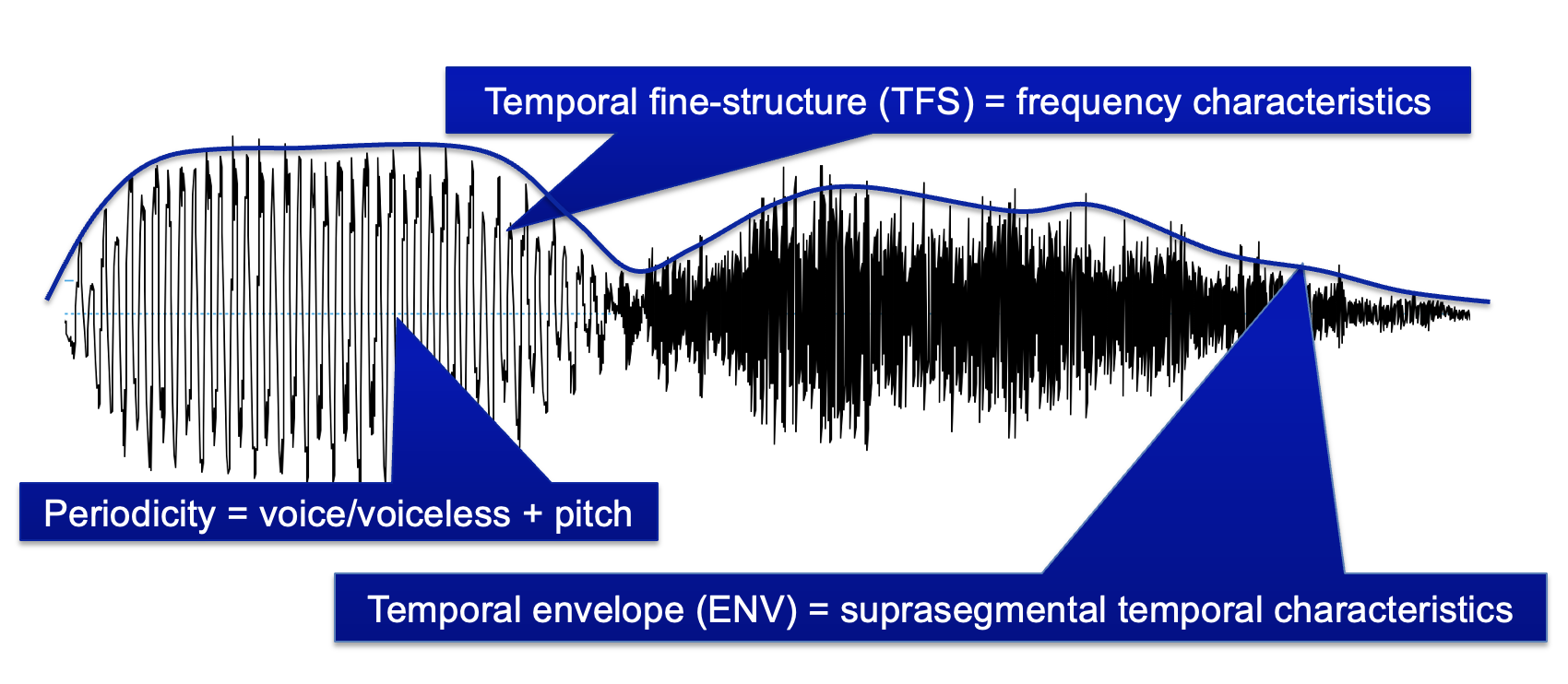
Rhythmic Variability in Swiss German Dialects
(Background image from slides of Prof. Dellwo Volker, 23 Spring, Fundamentals of Speech Science and Signal Processing)
Overview: This research explores the use of rhythmic metrics, specifically nPVI and VarcoV, in classifying Swiss German dialects from Basel, Bern, and Zurich. The results shows that nPVI and VarcoV are not suitable metrics for dialect differentiation.
Methods: Computation modeling in R, Linear Discriminant Analysis (LDA), Exploratory Data Analysis (EDA)
1. Introduction
1.1 Evolution of Speech Rhythm Research
The journey of speech rhythm research has been marked by significant shifts in understanding and methodology. Initially, the study of speech rhythm was heavily influenced by the rhythm-class hypothesis proposed by Pike in 1945[6] and Abercrombie in 1967[1]. They categorized languages into two rhythm types: stress-timed and syllable-timed rhythms. However, these early classifications, based largely on intuition, faced challenges as subsequent research in the 1970s and 80s failed to find clear empirical and acoustic evidence for these isochrony types. The acknowledgment of the challenges faced by early rhythmic classifications prompted a shift towards the phonetic-perceptual account. This framework has moved beyond the standard stress-timing and syllable-timing dichotomies, aiming to explicate the process of rhythm extraction from the speech signal and emphasize the role of timing variability in consonantal and vocalic speech intervals.
1.2 Rhythmic Metrics in Language Analysis
The pursuit of reliable acoustic correlates of rhythm has led to the development of new metrics. Two seminal contributions were the introduction of the percentage of vocalic intervals (%V) and the standard deviation of consonantal intervals (ΔC) by Ramus et al. in 1999[7], and the pairwise variability index (rPVI/nPVI) by Grabe and Low in 2002[4]. These metrics opened new avenues for quantifying and comparing rhythmic patterns across languages. For instance, it was observed that stress-timed languages typically exhibit a higher ΔC and a lower %V compared to syllable-timed languages. The application of these metrics revealed more nuanced and quantifiable differences between rhythmic classes, especially when incorporating a variation coefficient for ΔC (varcoC) proposed by Dellwo[3], which further enhanced the differentiation of rhythm classes in the analyzed data.
1.3 Focus on Swiss German Dialects
Related research has also been extended to the Swiss German dialect. Notably, Leemann et al.[5] conducted a comparative study on Swiss dialects derived from eight regions, and the results indicate that vocalic variability is a major discriminator between dialects and dialect groups, while rhythmic variability is complex and does not follow a uniform pattern across different dialects.
2. Research Questions
The distinct characteristics of Swiss German dialects offer an opportunity to explore how rhythmic metrics like nPVI and VarcoV can capture and differentiate intricate rhythmic patterns. As shown in Leemann et al.s research[5], there are significant differences between dialects in terms vocalic variability measured by ΔV, nPVI-V and VarcoV, along with consonantal variability measured by rPVI-C and nPVI-C. Among all metrics, nPVI and VarcoV were given special attention in the previous research since they yielded the highest number of significant post-hoc tests.
Based on a small corpus of Swiss German dialects in the region Basel, Bern and Zurich, this report aims to explore whether rhythmic metrics, specifically nPVI and VarcoV, can effectively classify these three Swiss German dialects. The central question revolves around the capability of these metrics to capture and distinguish the unique rhythmic characteristics of each of the three dialects.
3. Hypothesis
Using LDA, we can classify Swiss German dialects (Basel, Bern and Zurich) on the set of rhythmic metrics {nPVI_C, VarcoV}.
3.1 Null Hypothesis (H0)
The null hypothesis suggests that there is no statistically significant difference in the rhythmic patterns, particularly in terms of nPVI_C and VarcoV, among the three Swiss German dialects, implying that these dialects share similar rhythmic characteristics.
3.2 Alternate Hypothesis (H1)
Conversely, the alternate hypothesis argues that meaningful distinctions exist in the rhythmic patterns, specifically regarding nPVI_C and VarcoV, among the three Swiss German dialects. This implies that these dialects can be effectively differentiated based on their temporal speech production characteristics.
4. Feature Selection
4.1 Metrics Chosen
The metrics nPVI_C and VarcoV have been specifically selected due to their demonstrated efficacy in capturing rhythmic variations. The brief introductions are as follows:
- Normalized Pairwise Variability Index for consonantal intervals (nPVI_C): the mean of the differences between successive consonantal intervals divided by their sum, multiplied by 100[4].
- Variation Coefficient of vocalic interval duration (VarcoV): the standard deviation of vocalic interval duration divided by the mean vocalic duration and multiplied by 100[3].
4.2 Justification
The choice of these metrics is substantiated by previous research by Leemann et al.[5], which highlights their effectiveness in distinguishing between different Swiss German dialects, particularly the eastern and western dialects. By aligning our feature selection with their findings, we ensure a hypothesis-driven approach, concentrating on the features nPVI_C and VarcoV.
5. Pre-processing
5.1 Corpus Annotation
In pre-processing, Praat’s CV tier creator was used to annotate CV intervals in the corpus, categorizing segments into consonants and vowels. Consecutive segments were merged in the CVsegment interval tier, providing crucial boundary information in the CVintervals tier. Then the Duration Analyzer was used in Praat, extracting diverse metrics from the annotated CV intervals. This analysis encompassed metrics for consonantal (“C”), vocalic (“V”), and the amalgamation of both (“CV”). Two key metrics, nPVI_C and VarcoV, emerged as focal points in our study.
5.2 Data Splitting
To ensure robust model evaluation, a train-test split was implemented using an 80:20 ratio. The “dialect” variable guided the balanced partition creation, maintaining representativeness. The goal of this partitioning technique is to promote validity and generalization of the model.
5.3 Standardization
In the pursuit of consistent model performance, data standardization was applied. Parameters for standardization were estimated exclusively on the training data and then uniformly applied to both the training and testing datasets. Standardizing the features ensures that the model processes inputs consistently, mitigating biases stemming from varying scale magnitudes and enhancing overall model stability.
6. Modelling
6.1 EDA
Exploratory Data Analysis (EDA) was used to perform a detailed analysis of the regional distribution of VarcoV and nPVI_C first.
Outlier detection
Visualization of the typical data distribution sets the stage for the identification and management of outliers. Potential outliers were discovered when histograms were examined closely, leading to closer inspection. For nPVI_C, values surpassing 3.7 were deemed unusual, while VarcoV outliers were defined as values exceeding 4.0. To uphold data integrity, outliers were strategically addressed within the main dataset. Instances where nPVI_C exceeded 3.7 and VarcoV surpassed 4.0 were systematically replaced with NA values. This serves to enhance the robustness and reliability of subsequent modeling endeavors, reducing the impact of extreme observations.
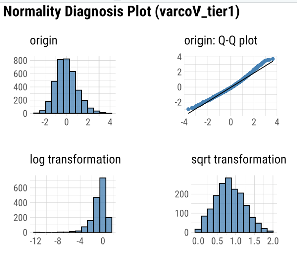
Figure 1: Normalization
Data transformation
Following outlier management, the next crucial step in EDA involves variable normalization and potential transformation. Diagnostic plots assessing normality were generated for both features. Upon evaluation, it was observed that the histograms did not indicate significant deviations from normal distribution. Preserving the original data’s normalization is important, so the decision was made to abstain from transformations, as they may distort the inherent normality of the data.
6.2 LDA
In this section the LDA model was trained to learn the classification task with the selected metrics nPVI_C and VarcoV on the train dataset, and evaluate the model’s performance on the test dataset.
LDA training and visualization
The Linear Discriminant Analysis (LDA) model’s training phase requires thorough data preparation. For both the training and testing sets, feature and response variables were defined, with non-feature columns excluded. The model was trained using the specified features from the training set. Here the training accuracy is 41.63%, which is the fraction of correct observations in the training data. Predictions derived from the training set were utilized to construct a scatter plot with ellipses, providing a visual representation of the dialect distribution.
LDA testing and visualization
The LDA model produced an accuracy of 43.06% when applied to the test set, meaning test data of this proportion were predicted correctly. Similarly, a scatterplot with ellipses was created based on the prediction results. The plot displays the predicted dialect labels as shapes and the true dialect labels as colors. Every point denotes an observation from the test set.
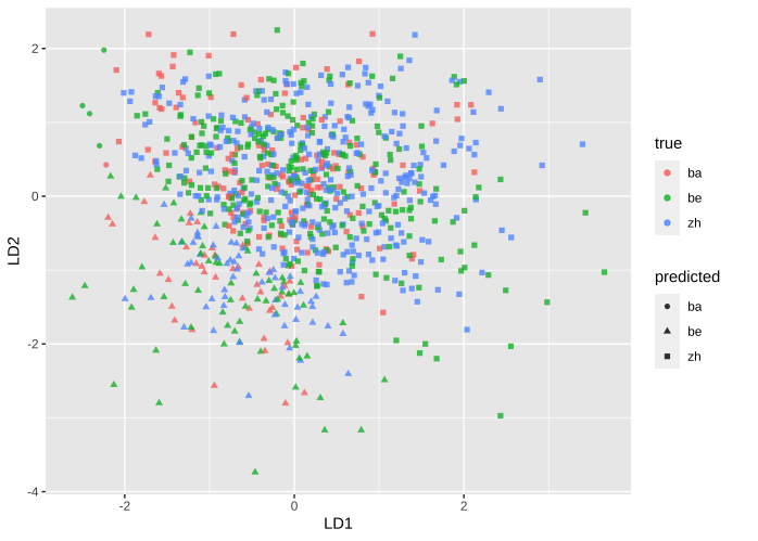
Figure 2: Scatterplot of Testset
7. Results
7.1 Confusion Matrix
| Prediction/Reference | BA | BE | ZH |
| BA | 1 | 4 | 0 |
| BE | 42 | 66 | 55 |
| ZH | 147 | 273 | 327 |
The diagonal elements are true positives of the predictions. For reference “BA”, the model performs poorly with only 1 correct prediction among 190 instances. The model achieves a higher number of correct predictions (66) for class “BE”, but it incorrectly predicts 4 instances as “BA” and 273 instances as “ZH”. For the data categories that make up the largest portion, the model performs way better with 327 correct predictions among all 382 instances.
7.2 Accuracy Score and Comparison with NIR
The overall accuracy of the LDA model on the test set is reported as 43.06%, with a 95% confidence interval (CI) of (0.3982, 0.4634). To provide a comprehensive evaluation of the model’s performance, a comparison is made with the No Information Rate (NIR). Considering the imbalanced nature of the dataset, the NIR is computed based on the major class, “ZH.”
NIR = Number of “ZH” data points / Total number of data points.
The accuracy of the model (43.06%) is slightly greater than the No Information Rate (41.75%), suggesting a slight improvement over a naive method of majority class prediction. P-value of the comparison between accuracy and NIR is 0.2202, exceeding the conventional significance level 0.05. It indicates that there is no statistically significant difference between accuracy and NIR. As a result, the accuracy gain might not be statistically significant compared with a baseline strategy of majority class prediction.
7.3 Class Specific Statistics
For the “BA” class, the model demonstrates subpar performance, with a Positive Predictive Value (Precision) of only 20.00% and a low Recall of 0.53%. The corresponding F1 Score is a mere 0.01. This indicates significant challenges in accurately identifying instances of the “BA” class. In contrast, for the “BE” class, the model achieves a Positive Predictive Value of 40.49% and a Recall of 19.24%, resulting in a relatively higher F1 Score of 0.26. Although an improvement compared to “BA,” it still reflects a moderate performance. It’s worth noting that the “ZH” class exhibits favorable Precision (43.78%) and high Recall (85.60%), yielding a rather robust F1 Score of 0.58. This signifies a better performance in identifying instances of the “ZH” class.
8. Discussion
Our analysis revealed that the model’s performance in classifying Swiss German dialects, especially for the “BA” and “BE” classes, was not as effective as anticipated. In contrast to the robust differentiation capabilities proposed by Leemann et al.[5] in Swiss German dialects, our study revealed more nuanced and less consistent classification success. This outcome aligns more closely with the Null Hypothesis (H0), suggesting that there are no significant differences in rhythmic patterns among the dialects that can be reliably captured by our chosen metrics.
The alignment with H0 leads to several potential counter-arguments into further consideration:
-
Dataset composition and representativeness: Our dataset, involving only 24 speakers, may not have encompassed the entire spectrum of rhythmic variability present in these three Swiss German dialects. A more diverse and comprehensive dataset with more speech samples could potentially yield different results.
-
Annotation criteria and consistency: The annotation process, carried out by three different researchers, might have introduced inconsistencies despite efforts to reach a consensus during uncertain cases. This variation in annotation could lead to discrepancies in the data, affecting the accuracy and reliability of the rhythmic metrics derived from the speech samples.
-
Appropriateness of Chosen Features: The specific metrics selected (nPVI_C and VarcoV) might not have been the most suitable for capturing the unique rhythmic characteristics of the dialects under our study. Exploring additional or alternative metrics could provide more insights.
-
Consideration of Language Varieties and Nuances: The effectiveness of metrics in classifying dialects might vary significantly across different language groups or dialect clusters.
-
Data Distribution and Alternative Modeling Approaches: The limitations of the LDA model and its moderate performance in this context suggest that the data distribution might not be ideal for linear discriminant analysis. Alternative modeling approaches (such as nonlinear classifiers or deep learning) could be further explored.
Apart from these, the research by Amalia Arvaniti[2] highlights the challenges and limitations associated with utilizing metrics for rhythm classifications in speech. The results indicate that individual differences play a significant role, potentially overshadowing broader linguistic patterns. Moreover, the susceptibility of metrics to methodological decisions underscores the influence of experimental design and data collection procedures on outcomes. The findings from the study by Wiget et al.[8] also emphasize the variability in rhythm scores attributable to differences in sentences, speakers, and measurers. Rhythm scores vary significantly between speakers, and the choice of sentences is a crucial factor affecting rhythm scores. Cross-linguistic comparisons and rhythmic categorization based on metrics are therefore inherently not robust. These studies remind us that these metrics are sensitive to a variety of extraneous factors, which should be taken into account when interpreting the results of the studies. In this way we can improve the accuracy and reliability of the results of speech rhythm and dialect studies.
References
[1] Abercrombie, D. (1967): Elements of general phonetics. Aldine: Chicago.
[2] Arvaniti, A. (2012). The usefulness of metrics in the quantification of speech rhythm. Journal of Phonetics, 40(3), 351-373. ISSN 0095-4470. https://doi.org/10.1016/j.wocn.2012.02.003.
[3] Dellwo, V. (2006). Rhythm and speech rate: A variation coefficient for deltaC. In: P. Karnowski, & I. Szigeti (Eds.), Language and Language-Processing: Proceedings of the 38th Linguistics Colloquium, Piliscsaba 2003 (pp. 231–241). Frankfurt am Main, Germany: Peter Lang.
[4] Grabe, E., & Low, E. L. (2002). Durational variability in speech and the rhythm class hypothesis. In: C. Gussenhoven, & N. Warner (Eds.), Laboratory Phonology 7 (pp. 515–546). Berlin: Mouton de Gruyter.
[5] Leemann, Adrian; Dellwo, Volker; Kolly, Marie-José; Schmid, Stephan (2012). Rhythmic variability in Swiss German dialects. In: 6th International Conference on Speech Prosody 2012, Shanghai, 22 May 2012 - 25 May 2012. ISCA, 607-610.
[6] Pike, K. L. (1945): The intonation of American English. University Press: Michigan.
[7] Ramus, F., Nespor, M., & Mehler, J. (1999). Correlates of linguistic rhythm in the speech signal. Cognition, 73, 265–292.
[8] Lukas Wiget, Laurence White, Barbara Schuppler, Izabelle Grenon, Olesya Rauch, Sven L. Mattys. (2010). How stable are acoustic metrics of contrastive speech rhythm?. J. Acoust. Soc., 127 (3): 1559–1569.**